Friday, September 18, 2009

July CPI: Steady As She Goes

There's been no real change on the inflation front over the last few months - the CPI has been climbing steadily at pretty much it's long term average. About the only thing of real note has been that m-o-m changes in the CPI have been positive for three months running, the first time that has happened since June-August 2008 (log monthly changes, 2000=100):


My rough and ready core inflation measure however is showing price rises slowing (remember this excludes food and transport):


Not that I'm too keen on the reliability of this measure. It turns out that BNM does indeed track core inflation, but they use multiple methodologies. The exclusion method as they call it, such as I'm attempting here, is the main instrument used but their choice of items on the exclusion list is obviously more refined than mine:


For anyone interested, the methodologies used are outlined in pgs 87-90 of last year's BNM annual report from which the chart above was reproduced, or you can download it directly here (warning: pdf link).

Friday, September 11, 2009

Gretl Tutorial IV: Seasonal Dummies

Links to Previous Tutorials:
Gretl Tutorial I
Gretl Tutorial II
Gretl Tutorial III

No, this isn’t about intelligence-challenged seasonal heretics. In my last few posts, I’ve pointed out the big difference in the picture presented by the raw economic numbers and that shown after seasonal adjustment – which neatly leads me to the purpose of the tutorial today. In my last post on using Gretl, the basic export forecast model I created showed some problems in the diagnostics, with both heteroscedasticity (time-varying variance) and serial correlation (non-independent error terms) present in the model. I identified two potential areas in the model specification that may require looking into: seasonal variation and a structural break. I’ll deal with modeling the seasonal variation first and structural breaks later.

First some concepts: to model seasonality as well as structural breaks, we use what are called dummy variables which take the value of 1 or 0. For instance, a January dummy would have the value of 1 for every January, and 0 for every other date. A structural break would have a value of 1 for every date before or after the date you think there is a break in the model, and 0 in every other date. Intuitively, the modeling procedure for seasonal dummies is that you are assuming that the trend is intact for the overall series, but that there are different intercepts for each month. For example, in the simple regression model:

Y = a + bX

we are assuming that there is a different value of a for every month. Structural breaks are harder, because you have the potential for a change in both the intercept as well as the slope, in other words both a and b could be different before and after the break. I’ll cover this in the next tutorial.

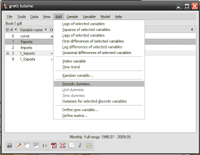
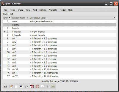
The actual procedure in Gretl is ridiculously easy. Load up the saved session from the past tutorials I covered (see top of this post), then select Add->Periodic dummies. Gretl automatically defines the variables for you in the session window:


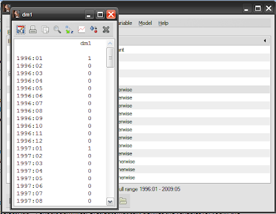
Just to be sure, double-click on the dm1 dummy, and verify that the values for January (denoted as :01) are all 1, and the values for other months are 0:


To create a new model using these new variables, open up the model specification screen by selecting from the session window Model -> Ordinary least squares:


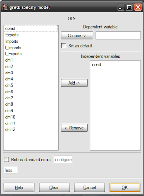
You now a choice to make – you can model seasonal variation as differences from a reference month, or directly as separate months. The choice is actually a question of whether you use a constant (variable const in the model specification screen) and 11 dummy variables, or drop the constant and use 12 dummy variables.

The estimation results will be exactly the same, except using the first approach lends itself to hypothesis testing monthly differences. I usually take the first approach because of this, which should give you the following specification (don’t forget to adjust the lag for imports to -1, per our original model):


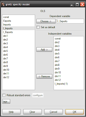
I’m using January as the reference month, so variable dm1 doesn’t have to be used. Finding the intercepts of each month is easy under this approach: just add the estimated coefficient for that month to the constant. You should get the following estimation results:


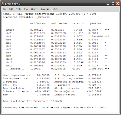
Looking at the p-values and stars on the right hand side (see this post for definitions), both the constant and the log of imports are statistically significant at the 99% level. Compare this with our original model:
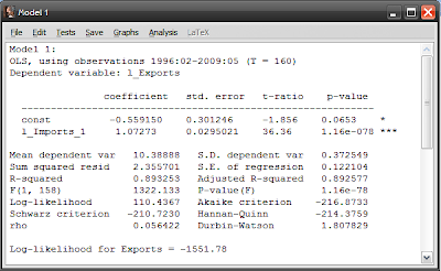


The intercept (the 
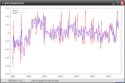
const variable) has fallen, while the slope (the coefficient for l_imports_1) has steepened. The R-squared number (the third row in the column of numbers below the results) measures how good a fit the model is with the data, with a value of 1 meaning a perfect match. R-squared in model2 has increased to 0.93 from 0.89 in model 1 – so our new model is a closer fit to the data, though not much more. Looking at the residuals (differences between the model and the actual data), our model 2 has gotten rid of some of the sharper spikes in the data, and the graph more closely approximates random noise (model 1 in red, model2 in blue):


Running through the diagnostics (see this post), it looks like I still have serial correlation and heteroscedasticity, but the distribution of the residuals is more “normal”:


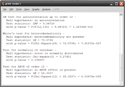
So the problems haven’t been solved by modeling seasonal variation, but we’ll leave that here to move on to seasonal adjustment.

The whole rigmarole of going through the above process is to illustrate some key concepts of seasonal adjustment mechanisms. By estimating the intercepts of each month, you can now construct a seasonal “index” – how different each month is to each other. A simple way to do this is to calculate each monthly intercept as a percentage of the average of all of them together. The resulting percentages can then be applied back to the data – you multiply each monthly data point by the index percentage for that month. Voila! You’ve now seasonally adjusted your data.

In practice, geometric averaging is preferred, and there’s also some modeling of business cycles which don’t necessarily follow a seasonal pattern. And since Gretl is a software package, it has the ability to do the whole thing for you although it does require you to add a separate third-party package.

Go back to the 
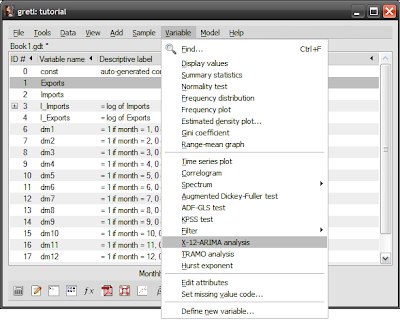
Gretl homepage, and you’ll see some downloads available as optional extras. The one’s you want are X-12-ARIMA and TRAMO/SEATS, which are used respectively in the US and Europe. Download and install either (or both), then save and restart the Gretl program. In the session screen, select the Exports series in the window, then select from the menubar Variable->X-12-ARIMA analysis (I found this to be really buggy, so save your session before and after you get the results):


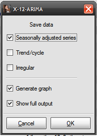
Click on the Save data: Seasonally adjusted series box and select Ok:


And you’ll get this nice graph:


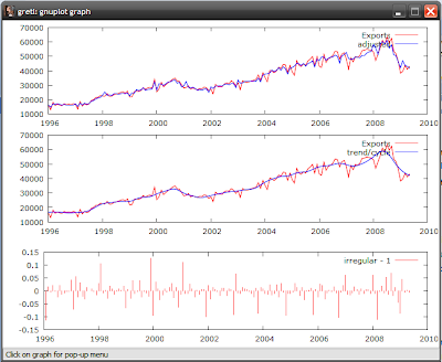
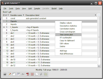
But more importantly, you get a new variable called Expo_d11 which is the seasonally adjusted series for Exports. You can do the same thing for imports, and rerun the models or just compare the series to see how different they are. To do the latter, just select any two series (like the export series), right click and select Time series plot:


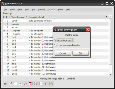
Choose your graph preference:
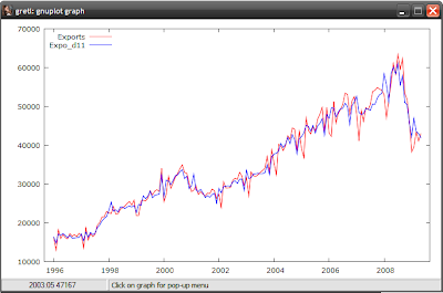


Which yields:


That’s it for today. Next up – breakdancing.

Thursday, September 10, 2009

July Industrial Production: Deceptively High

At first, I was pretty excited when I saw the numbers from today's IPI report (+6.9% m-o-m), especially coupled with US trade data for July which saw a surge in imports. Could my analysis be wrong (per my last post) and we are seeing a rebound in external demand? Sadly, digging deeper into the numbers, I'm forced to conclude there's insufficient evidence so far. The increase in US imports is real enough (seasonally adjusted, USD millions):


...and monthly growth confirms this (seasonally adjusted, log monthly changes):


...and at first blush, there's a corresponding increase in Malaysia's IPI level (2000=100) and growth (log monthly changes, 2000=100):


But adjusting for seasonal variations brings down both the IPI level (seasonally adjusted, 2000=100):


...and the growth rate (log monthly changes):


Looking at the detailed breakdown of US import data, again the numbers look to deceive. Nearly 60% of the increase of USD7 billion from July to June came from consumer goods and auto imports. A further USD1 billion came from crude oil imports and another USD500 million in imports of computer equipment.

The problem is that the US government "cash for clunkers" program is probably the main driving force behind both the increases in auto and oil imports, and H1N1 may be behind the more than USD1 billion increase in pharmaceuticals (which is under the consumer category).

Take away those two factors and US import growth actually falls behind export growth. Since neither are expected to have long term effects, it's difficult to make an argument that there has been a meaningful change in consumer spending patterns - in short, we're not seeing a long term resumption of US import demand.

So I'm back to my inventory bounce/domestic demand story...for now.

Technical notes:
1. July IPI data from the Department of Statistics
2. US trade data from the Bureau of Economic Analysis

Tuesday, September 8, 2009

July Trade: My Crystal Ball Is Murky

Malaysia's trade is slowly improving, even if the yearly growth numbers are still in the negative (log annual changes):


Headline exports increased 8.1% m-o-m, but most of this increase is seasonal:


After seasonally adjustment, m-o-m growth actually slowed for both exports and imports (log monthly changes):


My initial reaction to these numbers were that we were finally seeing some real recovery in external demand, but looking deeper at the data I'm not too sure now. The export numbers beat my model point forecasts handily, although still within forecast confidence intervals. But one thing that is catching my eye is that imports have recovered quicker than exports.

There are two things I can think of that may be causing this. First is my original thesis that we're in the middle of an inventory correction, and exporters are rebuilding stocks depleted in the past year. By cutting production drastically and reducing inventory, exporters conserved cash until they could see some signs of a return to economic normalcy, as is happening now. That would explain the divergence between exports and the relatively faster recovery in imports of intermediate goods:


...while capital goods imports have also yet to fully recover, implying a slower increase in capacity:


But what could have the same effect on imports would be if domestic demand was increasing faster as well. Why I'm thinking this is the unseasonal increase in private consumption embedded in the 2Q GDP data, and the fact that consumption imports have held up relatively well:


Quite possibly we're looking at both effects here. Another reason why I'm less than convinced about the return of external demand is the relative strength of the Ringgit in recent months, which may be inflating export values and overstating export volume.

It hardly matters from a recovery standpoint whether domestic or external demand is driving recovery, but over the longer term the former may signal structural changes in the economy.

Next month's predictions:

Seasonally adjusted model:


Point forecast:RM46743, Range forecast:RM52546-RM40940

Seasonally effect model:

Point forecast:RM51644, Range forecast:RM57784-RM45504


Technical Notes:
July trade data courtesy Matrade.

Thursday, September 3, 2009

National Debt Update

I haven't covered this topic in a while, so with the government's borrowing program now in full swing, an update is timely.

The federal government's fiscal balance has been negative now since 2Q 2007 (RM millions):


Because expenditure has largely kept track with revenue, the deficit has largely been due to an increase in net development expenditure. The trends are even clearer on a seasonally adjusted basis (RM millions):


An obvious culprit is petrol subsidies, which the latest statements by the Minister of Domestic Trade and Consumer Affairs suggest is running at RM304 million a month for the newly introduced RON95 fuel alone - I'd guess that total petrol subsidies would be in the region of RM400+ million when all is said and done, but that doesn't include the subsidies for diesel, or the hidden subsidy for natural gas which is paid for by Petronas. Total annual cost at current crude oil price levels will therefore be over RM5 billion, or rather more than the country is paying for national healthcare - talk about misplaced priorities.

But development expenditure has accelerated far beyond those levels, which we can probably partly attribute to the two stimulus packages, as well as the planned deficit spending already incorporated in this year's budget. Government borrowing really ratcheted up in February this year, but that was mostly due to the need to meet maturing MGS and GII issues. On a net basis, borrowing didn't really accelerate until May, when a net RM13.8 billion was tapped from the local market:


Up to the end of 2Q 2009, the national debt stood at RM335.7 billion, the bulk of which (RM 228 billion) comprised MGS:


A further RM18 billion was tapped in July and August (gross: I'm not sure how to check on redemptions for August), which brings the grand total to RM353 billion. I'm expecting the rate of borrowing to continue at this pace for most of the rest of the year, and we should see the total to stand at around RM375-380 billion by the new year.

The fiscal deficit has of course continued to deteriorate (4-quarter moving average; ratio to nominal GDP):


...as has the Debt to GDP ratio (4-quarter moving average; ratio to nominal GDP):


The end result is also a significant increase in debt per capita (nominal RM, projected line based on RM380 billion):


My original estimate was that we would see debt per capita reaching RM13,500 inclusive of the two stimulus packages - based on the current rate of borrowing, we're going to see that by the end of this year.

Technical Notes:
1. Federal Government finance and public borrowing data from BNM's MSB
2. August public borrowing data from FAST

Wednesday, September 2, 2009

July 2009 Monetary Policy Update

I'm scratching my head over some of the developments in interest rates - there are some minor divergences in what I'm expecting against what the markets are doing. But first, growth in monetary aggregates have stabilised over the past couple of months, which should be no surprise given there's been no change in the OPR and the signals BNM has been giving out (log annual changes):


Under the current circumstances, there should be no movement in the policy rate until at the very least mid-to-early next year. That hasn't stopped some gyrations in market interest rates however. Average lending rates are down 8bp through the end of July, which has dropped the spread over overnight rates to just under 3%:


Loan growth as a result has accelerated on a m-o-m basis (log monthly changes, annualised):


The good news is that most of July's increase came from working capital loans, and that the increase is across a broad swath of sectors (but particularly in education and health). This suggests that activity is picking up particularly in domestic oriented sectors, which is exactly the kind of recovery driver we need going forward. NPL ratios at both 6-month and 3-month spans have continued to drop:


I was actually expecting loan defaults to pick up this quarter, as it's been long enough from the onset of the crisis for marginal firms to start going to the wall. Turns out Malaysian companies may be more resilient than expected.

Turning to the bond markets, it's MGS yields that have me puzzled - despite a net increase of RM9.5 billion in government domestic borrowing in July, the yield curve has flattened at the long end:


What makes this even more puzzling is that the July issues (RM8.5 billion in 10yr MGS, and RM4.5 billion in 5yr GII) are all long dated. Anyone care to venture an explanation? Because I haven't any ideas at the moment. An increase in bond supply should ceteris paribus drop prices, which should in turn increase yields. An alternative answer is that MGS demand has also picked up in the interim which may be a factor of an increase in foreign demand, although I'm stumped why the action should happen at the long end rather than at the shorter tenures. A possible change in market risk appetite?

Tuesday, September 1, 2009

Big Macs Again

*Sigh*

The Economist states upfront (with tongue firmly in cheek) that the Big Mac Index is "a lighthearted guide to valuing currencies" and "It is arguably the world's most accurate financial indicator to be based on a fast-food item."

The joke here is that it's the only financial indicator based on a fast food item.

The Star however apparently takes this seriously:

"According to the latest Big Mac Index, arguably the world’s most accurate financial indicator to be based on a popular burger, most Asian currencies are undervalued against the US dollar.

The ringgit is undervalued by 47% against the greenback, which was at the same level as the Thai baht.

Only Hong Kong (52%) and China (49%) were lower than Malaysia and Thailand among Asian countries."


I've ruminated on this subject before, and I'm not inclined to go through it again - but PPP-based exchange rate measures are simply not an empirically valid way to evaluate exchange rate levels or movements.