Gretl Tutorial III: Diagnostics – “He’s dead, Jim”

Gretl Tutorial I

Gretl Tutorial II

Now that we have a decent regression that seemingly outlines a plausible relationship between exports and lagged imports, we have to test from a statistical perspective whether we can make inferences from the resulting equation. That will determine whether we can actually make statistically reliable forecasts. So what are the potential problems we can encounter?

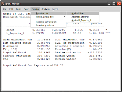
Papering over an academic discussion of the properties of estimators, from a simplistic perspective what we are trying to achieve is a model where coefficient estimates are unbiased, efficient, linear and consistent. This is actually best achieved not by looking at the estimators themselves but by looking at the residuals, which is the difference between the actual data and the estimated relationship. You can get view the residuals in Gretl by looking at the results screen, selecting Graphs->Residual plot->Against time:




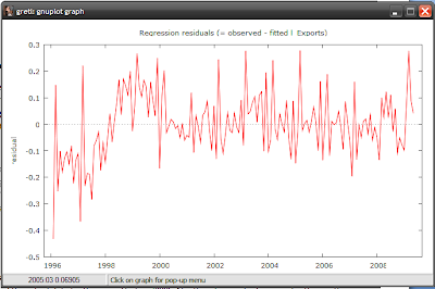
A cursory examination of the residuals is revealing. As I noted earlier, there’s a discontinuity between our results and the actual data for the period before 2000. Also there’s a marked seasonal pattern in the residuals, which means seasonality is a factor as well. But I’m leaving that for the next post, which will deal with dummy variables. For now, I want to look at some of the standard diagnostic tests that are typically used to make sure our model is a valid one.

The two main problems with times series deal with the requirement that residuals must be independent and normally distributed:

1. Serial correlation – which means residuals are not independent over time, and are in fact correlated;

2. Heteroscedasticity – which means variance (and standard errors) are not constant, and thus residuals are not normally distributed.

There are a number of standard statistical tests that can be performed to find out whether either of these two conditions hold; if they do, then we have to rethink our model.

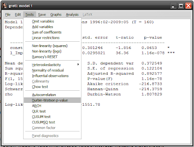
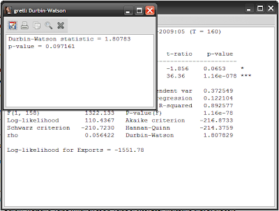
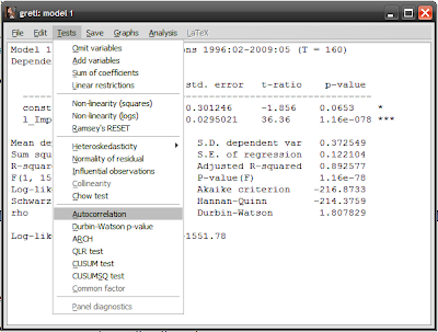
The most common method to test for serial correlation is one you don’t have to perform; both Gretl (and EViews) report the Durbin-Watson statistic as part of the estimation results. In the Gretl results screen, it is the last number reported in the right column, with a value of 1.807829. The actual test statistic requires some calculation but essentially a value of 2 means no serial correlation, while a value of 4 or 0 mean perfect positive or negative correlation. As a short cut, in the results screen you can select Tests->Durbin-Watson p-value which gives a p-value of 0.097161, indicating that at the 95% confidence level you cannot reject the null hypothesis of no serial correlation:




Unfortunately the DW stat has a weakness in that it is only a valid test for serial correlation over 1 lag. For multiple lags, you need to use a different test. The Breusch-Godfrey test allows for this and can be reached at Tests->Autocorrelation (I’m using 12 lags here):




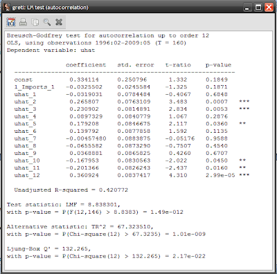
As you can see, while the BG test echoes the DW stat for the first lag, there is serial correlation at lags 2, 3, 5, 10, 11, and 12 (check the stars). All the test statistics (at the bottom of the test results page) show very small p-values, indicating a rejection of the null hypothesis of no serial correlation. Note that any tests you do are automatically added to the results page, below the estimation results – a nice touch.

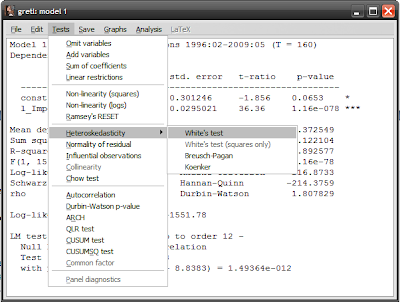
To test for heteroscedasticity, select Tests->heteroskedasticity (sic)->White’s test:




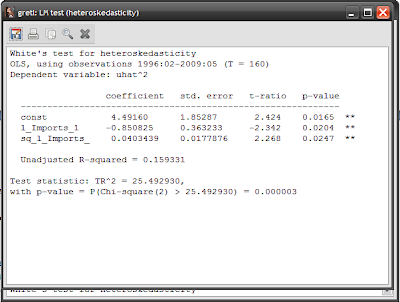
The p-value is 0.000003, which means you have to reject the null hypothesis that there is no heteroscedasticity.

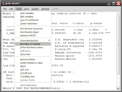
As an additional test, you can directly test whether the residuals are normally distributed (select Tests-> Normality of residual):





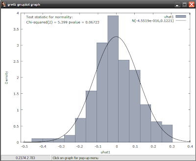
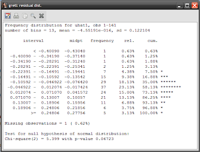
The p-value of 0.06723 means that it's a close run thing - you would accept the null hypothesis of normality at the 95% confidence level, but reject it at the 90% confidence level.

Lastly, I almost always test for ARCH (select Tests->ARCH):



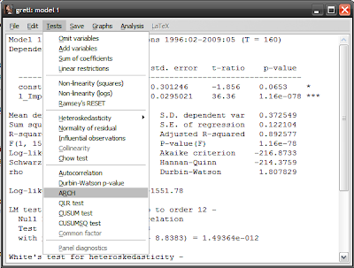
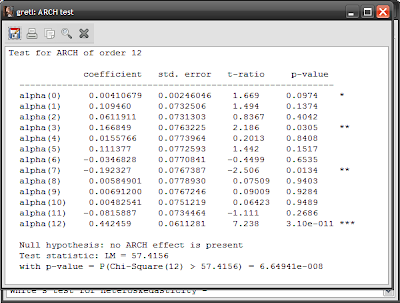
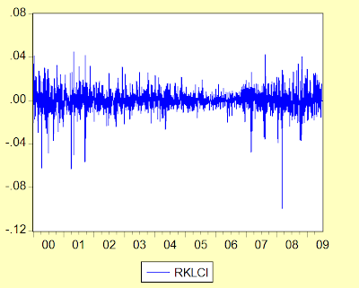
Which suggests that ARCH is present as well. ARCH is a special form of heteroscedasticity – it’s an acronym that means auto-regressive conditional heteroscedasticity, and is especially common in financial markets. It’s also a rather fancy way of saying that volatility clumps together, as illustrated by this chart of daily log returns on the KLCI:



Going back to our trade model, we have some very obvious problems. With both heteroscedasticity and serial correlation present, I’d be very wary of relying on the model as it stands. To solve this, we need to relook the model specification – the pattern of residuals provides the main clue. We have to deal with seasonality, and we have to deal with a potential change in the relationship between exports and imports post-2000.

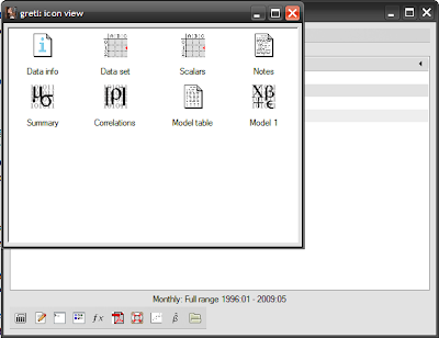
But before moving on, you can save the work you’ve done by selecting File->Save to session as icon, and then saving the session. The next time you start Gretl, select File->Session files->Open Session, then select the name of the session file you saved your work under, and your work will automatically be available through the session window under an icon named “Model 1”: