Gretl Tutorial IV: Seasonal Dummies

Links to Previous Tutorials:
Gretl Tutorial I
Gretl Tutorial II
Gretl Tutorial III

No, this isn’t about intelligence-challenged seasonal heretics. In my last few posts, I’ve pointed out the big difference in the picture presented by the raw economic numbers and that shown after seasonal adjustment – which neatly leads me to the purpose of the tutorial today. In my last post on using Gretl, the basic export forecast model I created showed some problems in the diagnostics, with both heteroscedasticity (time-varying variance) and serial correlation (non-independent error terms) present in the model. I identified two potential areas in the model specification that may require looking into: seasonal variation and a structural break. I’ll deal with modeling the seasonal variation first and structural breaks later.

First some concepts: to model seasonality as well as structural breaks, we use what are called dummy variables which take the value of 1 or 0. For instance, a January dummy would have the value of 1 for every January, and 0 for every other date. A structural break would have a value of 1 for every date before or after the date you think there is a break in the model, and 0 in every other date. Intuitively, the modeling procedure for seasonal dummies is that you are assuming that the trend is intact for the overall series, but that there are different intercepts for each month. For example, in the simple regression model:

Y = a + bX

we are assuming that there is a different value of a for every month. Structural breaks are harder, because you have the potential for a change in both the intercept as well as the slope, in other words both a and b could be different before and after the break. I’ll cover this in the next tutorial.

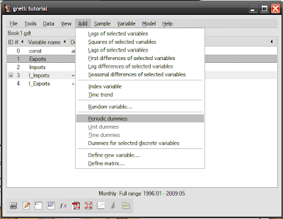
The actual procedure in Gretl is ridiculously easy. Load up the saved session from the past tutorials I covered (see top of this post), then select Add->Periodic dummies. Gretl automatically defines the variables for you in the session window:




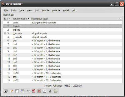
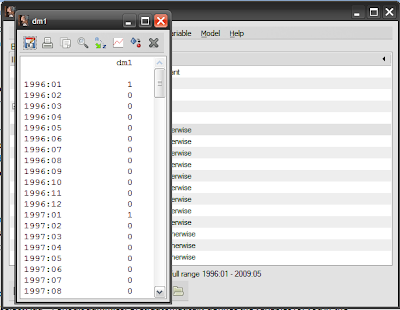
Just to be sure, double-click on the dm1 dummy, and verify that the values for January (denoted as :01) are all 1, and the values for other months are 0:



To create a new model using these new variables, open up the model specification screen by selecting from the session window Model -> Ordinary least squares:



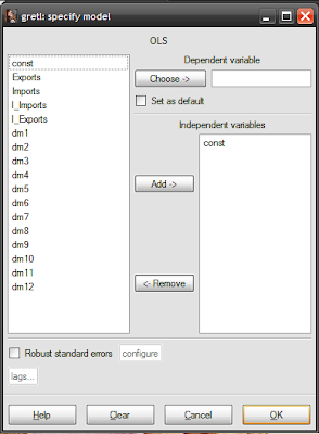
You now a choice to make – you can model seasonal variation as differences from a reference month, or directly as separate months. The choice is actually a question of whether you use a constant (variable const in the model specification screen) and 11 dummy variables, or drop the constant and use 12 dummy variables.

The estimation results will be exactly the same, except using the first approach lends itself to hypothesis testing monthly differences. I usually take the first approach because of this, which should give you the following specification (don’t forget to adjust the lag for imports to -1, per our original model):



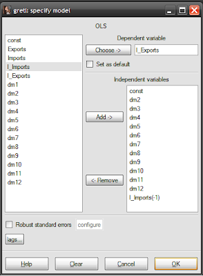
I’m using January as the reference month, so variable dm1 doesn’t have to be used. Finding the intercepts of each month is easy under this approach: just add the estimated coefficient for that month to the constant. You should get the following estimation results:



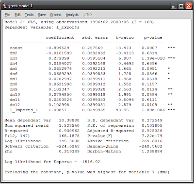
Looking at the p-values and stars on the right hand side (see this post for definitions), both the constant and the log of imports are statistically significant at the 99% level. Compare this with our original model:



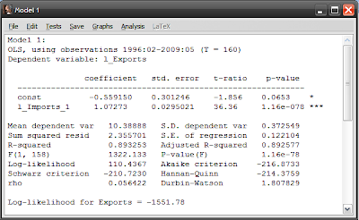
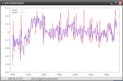
The intercept (the const variable) has fallen, while the slope (the coefficient for l_imports_1) has steepened. The R-squared number (the third row in the column of numbers below the results) measures how good a fit the model is with the data, with a value of 1 meaning a perfect match. R-squared in model2 has increased to 0.93 from 0.89 in model 1 – so our new model is a closer fit to the data, though not much more. Looking at the residuals (differences between the model and the actual data), our model 2 has gotten rid of some of the sharper spikes in the data, and the graph more closely approximates random noise (model 1 in red, model2 in blue):



Running through the diagnostics (see this post), it looks like I still have serial correlation and heteroscedasticity, but the distribution of the residuals is more “normal”:



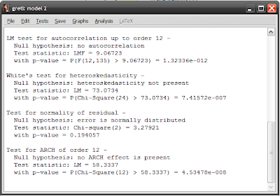
So the problems haven’t been solved by modeling seasonal variation, but we’ll leave that here to move on to seasonal adjustment.

The whole rigmarole of going through the above process is to illustrate some key concepts of seasonal adjustment mechanisms. By estimating the intercepts of each month, you can now construct a seasonal “index” – how different each month is to each other. A simple way to do this is to calculate each monthly intercept as a percentage of the average of all of them together. The resulting percentages can then be applied back to the data – you multiply each monthly data point by the index percentage for that month. Voila! You’ve now seasonally adjusted your data.

In practice, geometric averaging is preferred, and there’s also some modeling of business cycles which don’t necessarily follow a seasonal pattern. And since Gretl is a software package, it has the ability to do the whole thing for you although it does require you to add a separate third-party package.

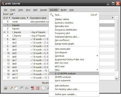
Go back to the Gretl homepage, and you’ll see some downloads available as optional extras. The one’s you want are X-12-ARIMA and TRAMO/SEATS, which are used respectively in the US and Europe. Download and install either (or both), then save and restart the Gretl program. In the session screen, select the Exports series in the window, then select from the menubar Variable->X-12-ARIMA analysis (I found this to be really buggy, so save your session before and after you get the results):



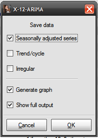
Click on the Save data: Seasonally adjusted series box and select Ok:



And you’ll get this nice graph:



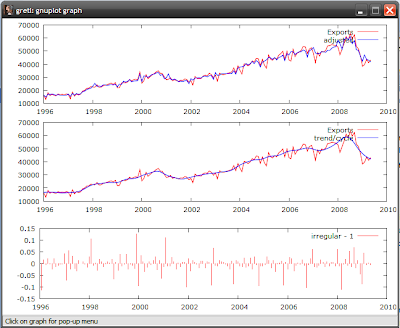
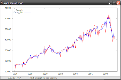
But more importantly, you get a new variable called Expo_d11 which is the seasonally adjusted series for Exports. You can do the same thing for imports, and rerun the models or just compare the series to see how different they are. To do the latter, just select any two series (like the export series), right click and select Time series plot:



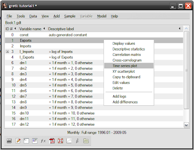
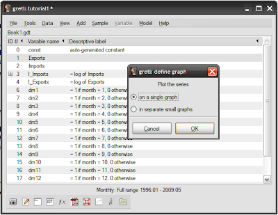
Choose your graph preference:



Which yields:



That’s it for today. Next up – breakdancing.