Gretl Tutorial II: OLS Regression

Gretl Tutorial I

Now that we have a dataset to play with, what can we do with it?

I based my simple trade models on the assumption that Malaysian imports and exports are cointegrated i.e. that there is a long term relationship between the two variables.

Intuitively, since 70%+ of imports are composed of intermediate goods, which are goods used as inputs into making other goods (including exports), we would expect a statistically significant relationship between exports and imports. For instance, exporters would have certain expectations of demand (advance orders) and order inputs based on that demand. After processing, the finished goods would then be exported.

In such a case, imports of inputs would lead exports by a time factor, depending on the length of time engaged in processing. This is something we can actually test, but I’ll leave that for later and just assume a lag of 1 month. Since imports are based on expected future export demand, we can then use imports to actually forecast exports.

There are some problems with making such a simplistic assumption of course (e.g. how do we account for exports with no foreign inputs), but since this is a demonstration of regression analysis and not an econometric examination of the structure of Malaysian trade, we’ll ignore it for now. In any case, for forecasting purposes, structure (economically accurate modeling) is less important than a usable and timely forecast.

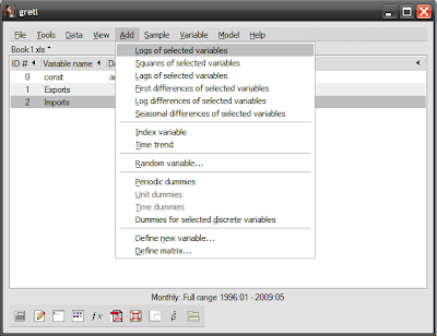
If you’ve gone through the previous post, you’ll have export and import data loaded into Gretl and ready to go. The first step is to transform the data to natural logs. Select both variables (Ctrl-click), then go to the menubar and click Add->Logs of selected variables:



You’ll now have two additional variables called l_imports and l_exports:



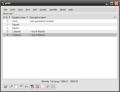
The reasons we transform into natural log form is twofold: most economic time series are characteristically exponential with respect to time, and a log transformation changes the vertical scale to linear. Log transformations also make elasticity calculations easier, as the estimated coefficients are approximate to percentage changes in the variables.

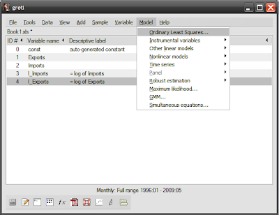
To estimate the regression, click Model->Ordinary least squares…:



…which will give the model specification screen:



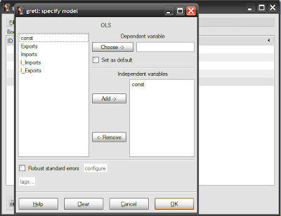
Select l_exports then click on the “Choose” button, which sets the log of exports as the dependent variable. Then select l_imports and click the “Add” button, which sets the log of imports as the explanatory variable. At this stage, you should note that the “lags…” button turns from greyed out to normal. Click on this, which brings up the lag screen:



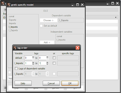
Set the l_imports lag to 1 in both boxes, then click “Ok” and “Ok”.[1] You’ll now get the results window:



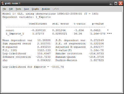
Don’t worry if the results window looks complicated, there’s only a few numbers that you really have to deal with...for now. First are the results of the estimation itself:

(l_exports)=-0.551950+1.07273(l_imports(-1))

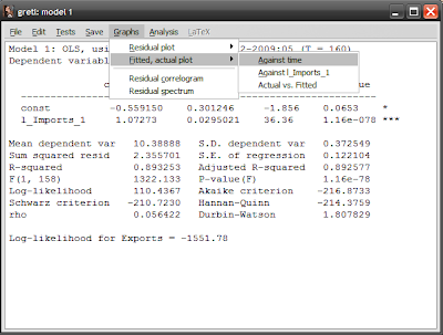
The interpretation here is that a 1% rise in last month's imports causes a 1.07% rise in this month's exports. To have a look at your work, click Graphs->Fitted, actual plot->Against time, in the results window:



You should see this:



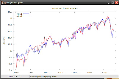
The red line displays actual values of l_exports, while the blue line represents the values from your estimated equation. Note that before 2000 the forecast errors are fairly large compared to after 2000, both under- and over-estimating exports. On the whole however, the results of the equation looks good, and seems to be a fairly accurate forecast model for exports.

Now, that wasn't so hard was it?

But we still have to be sure that this is a statistically significant relationship. Ordinarily, this involves a hypothesis test of the coefficients (null hypothesis=0), which involves using the standard errors to calculate a T-ratio, which is then evaluated against the critical values in a Student's T table.[2]

Since busy people can’t be bothered with stuff like that, Gretl very nicely lets you skip all those steps – all you have to pay attention to is the p-value. I could give a technical explanation for what it is, but all you have to know is that [1-(p-value) x 100] gives the confidence level. So if the p-value is 0.05, then you are 95% confident that the estimated coefficient is statistically significantly different from zero (statistically significant for short).

You can skip even this step, and just look at the stars Gretl appends on the right side of the p-value. One * means a 90% confidence level, ** means a 95% confidence level, and *** means a 99% confidence level. Just like hotels and restaurants, the more stars the better.

In the case of this estimation, we are 93.5% confident that the constant is statistically significant and 99.999% confident that the coefficient for l_imports is statistically significant.

You now have what appears to be a decent model for estimating future exports, at least for a 1-month ahead forecast. But since forecasting can’t be obviously so simple, we’ll look at some of the necessary tests to do to confirm we have a econometrically solid model to rely on.

[1] You can skip this step by directly specifying the lagged data series in the session screen. Select the variable you want then click Add->Lags of selected variables, then select the number of lags you want. Then in the model screen, select the lagged variable as the explanatory variable, rather than the original explanatory variable. Whether you take this step or the one I explained above, a lagged data series will be added to your dataset.

[2] You can do this manually within Gretl if you’re masochistic. The critical values can be accessed in the session screen, by clicking Tools->Statistical Tables, then selecting “t” from the tabs. Put value 160 in the “df” (“degrees of freedom”) box, and 0.025 in the “right-tail probability” box which corresponds to a two-tail 95% confidence level test. You should get a critical value of 1.9749. Since the constant has a t-ratio of -1.856, it is not statistically significant, but the coefficient for l_imports has a t-ratio of 36.36 which means it is at the 95% confidence level. You can vary the value for the “right-tail probability” box to obtain the critical values for other confidence levels.