This Isn’t The Purpose Of Government

From today’s Star (excerpt):

Sugar supply to be increased from Thursday

The Government will add 10% more sugar supply to wholesalers and retailers nationwide from this Thursday until September, said Domestic Trade, Cooperatives and Consumerism Minister Datuk Seri Ismail Sabri Yaakob.

"The additional supply is to meet the high demand for sugar, especially during the coming festive season," he said when winding up the debate on the 10th Malaysia Plan for his ministry in the Dewan Rakyat, here, Tuesday.

Early this month, the Government added 5% to the sugar supply to meet the current demand.

Ismail Sabri said to ensure sufficient sugar supply always, the Government had appointed the relevant associations to supply and distribute the essential commodity to their members.

The government has a positive role in lot of things that impact society, from healthcare, to defense, to education – but acting as a sugar daddy shouldn’t be one of them.

Sadly this is a major consequence of having administered prices – because the tendency is to set prices below the market clearing level (and ours is somewhere about a third below that level), you’re always ending up with a shortfall in production and supply. Which in turn means spending money on securing an imported source to cover the deficit. The flip side of that is because sugar is cheaper than it should be, consumption is also higher than it should be.

The problem with sugar is that, unlike salt, it’s really hard to figure out if you’re taking too much. So this higher consumption is in part going towards over-sweet processed foods, which in all probability would probably taste just as good with less sugar in the mix.

From a socio-economic perspective, the subsidy and price controls on sugar are indefensible. Let’s get rid of them now, please. And while we’re at it, let’s slap a tax on sugar that would help cover its true economic cost in helping foster obesity, diabetes, heart disease and high blood pressure.

IMF Finance & Development Magazine Focuses On Asia

The June issue is worth a read, as it covers many of the broad policy challenges that Malaysia must overcome: from financial sector regulation, to the shift to domestic demand/services-led growth, to national debt reduction.

I was struck by this passage however in the article on the services sector (which, by the way, is highly relevant to Malaysia and our 2020 goal):

“ARCHANA NANANCHERLA attributes India’s economic success to her compatriots’ appetite for hard work. 'We work harder than others . . . it is a trait of Indians,' she declares. But perhaps it is Nanancherla herself and people like her—educated, working in the service sector, with growing disposable income—who are the real secret behind India’s domestic-led growth."

There’s more than an echo here in the first part of the quote above, of the hubris coming out of parts of East Asia (including ourselves) in the mid-1990s – the “East Asian Miracle”, and the superiority of “Asian culture” and “Asian values”. Nor is this an isolated opinion, as I see similar attitudes online, especially among younger Indian and Chinese nationals.

I hope India (and China) never have to go through what we experienced a decade ago, though in India’s case I’m not too optimistic.

More On Measuring Inflation

In The Star today, Dr Fong Chan Onn says we need to make the CPI more “realistic”:

Figures that matter

MUCH has been articulated about how the Consumer Price Index (CPI) is not reflective of the purchases of ordinary Malaysians any more. This is especially true for the low to middle income wage earners, where the bulk of the population sits.

The reported CPI in Malaysia has been increasing by about 3% per annum for the last three decades, while the world CPI has gone up 3,000 times over the same period (see table on the far right). So much so that housewives scoff when they are told that prices of goods and services are only increasing at 3% a year...

...It also makes the ordinary citizens think that politicians and policy-makers are completely disconnected from the realities of Malay­sian life, cocooned in making decisions that do not reflect the hardship they have to bear.

Employers and trade unions, when making yearly adjustments to wage levels, use the CPI as the basis for salary increments. Trade unions’ grouses are justified in the case of arguing that wage levels are not enough for a typical household to survive. However, they are equally frustrated with the system, as there is no other index or basis for greater wage increments...

...“Food and non-alcoholic beverages” and “Housing, water, electricity, gas and others fuels” make up over 52.8% of the weightage. Without going into the finer details of what the actual items are in these two categories, it is suffice to say that most of the items are either heavily subsidised or price controlled, like sugar, flour, water, petrol, electricity and so forth.

The dislocation in the CPI and the real prices paid by a household becomes more obvious when we consider that we do not just consume flour and sugar in its raw form, but in value-added items like cooked food and beverages. Eating out in coffee-shops or warung certainly include prepared items such as cooked fish, vegetable and prawns which are always levied at market prices but not captured in the CPI.

Transport, which makes up 15.9% of the weightage, does not take into account hire purchase for cars or motorcycles or the cost of imported spare parts for their repair.

Construction materials such as cement and clinker may be price controlled but the prices of houses and rental are determined at market rates, which are not subjected to regulations.

Mobile devices have become an integral part of our daily lives. Most of us have to pay bills for SMS, telephone calls and data download that are not included in the communication category.

The impact of an artificially low inflation rate is as follows:

> Important business decisions are based on the inflation rate, and this can mislead the private sector into making business judgments that are off the mark, costing the economy billions in losses.

> It leads to wages being artificially suppressed, creating a widening income gap between Malaysians working domestically and those working outside the country. This, in turn, exacerbates the “brain drain” problem.

> With low wages, we are not able to attract outside talent into Malaysia even though our goods and services are supposedly cheaper.

> It creates a technology gap, making Malaysia uncompetitive. Technology goods and services become expensive for Malaysians to purchase, including things like iPhones, Blackberry, and iPads which are soon becoming everyday items.

> We will have to depend on a low foreign exchange rate to ensure that Malaysian goods remain competitive but this is an unsustainable strategy in the long run.

> With a cheap currency, we cannot afford to purchase the most advanced machinery and technology, leading to poor fixed asset/capital build-up. This also explains part of the problem of sluggish private sector investments.

The implication of having an unrealistic CPI is a very serious matter and cannot be brushed aside as mere grumblings of the rakyat. However, just like in the treatment of the removal of subsidies and price controls, proper safety nets must be in place to protect the lower income and vulnerable groups.

The general price levels of the basket of goods and services will no doubt adjust itself as subsidies and controlled items are subsequently removed but this has to be done gradually to prevent hyper-inflation.

And additional items such as communication devices and computers will have to be introduced to reflect a more competitive and advanced Malaysia.

Next to the Gross Domestic Product (GDP), the CPI is probably the most important economic indicator that all governments use to gauge the health of an economy. As the CPI is the basis of many policy benchmarks with very far-reaching implications in the management of an economy and the wealth of a nation, a strong case of a more realistic mechanism for the computation of CPI is timely and much needed in an open and globally connected economy like Malaysia.

Included in the print version (not reproduced online) are a table of the CPI weights and a chart showing the different price levels as measured by the CPI of the world and Malaysia from 1980 to 2008. You can peek at the former in the May 2010 CPI report here. For the latter, no sources were listed, which is really vexing as it doesn’t allow for verification.

So I’ve done my best to reproduce it from data in the IMF World Economic Outlook database (estimated CPI levels, 1980=100):

It’s a pretty close approximation to the chart in print, and if anything shows an even greater difference between Malaysian and global inflation – the global price level in 2008 is 31.4x higher than in 1980, while the Malaysian price level is just 2.3x higher.

So that must mean that Malaysia’s CPI is a farce, right? Not so fast.

There’s a few ways to spin this. First is a presentation trick (one I was warned about while doing my Masters thesis) – change the base year, and your data plot and your appreciation of what it says will be completely different. So what happens if we change the base year to 2000, which is the current internationally accepted standard?

While the Malaysian price level is still increasing at a slower pace than the global price level, the comparison doesn’t look quite as stark.

Going further back, the big jump in the global price level occurred circa 1990-1994, and began accelerating around 1988. Off the top of my head, there are three events occurring in that time span that probably boosted world inflation in general, some which impacted Malaysian inflation and some which did not:

1. The Plaza Accord (1985) – a coordinated action to depreciate the USD relative to global currencies. This had the effect of boosting commodity prices in USD terms for a decade, as the coordinated devaluation of the USD relative to other major currencies didn’t cease with official intervention, but continued until approximately 1995:
   
   
   
2. The 1st Gulf War (1990-1991) – the Iraqi invasion of Kuwait in August 1990, and the subsequent US-led coalition liberation effort in Jan-Feb. Beyond the socio-political impact of the war, oil prices spiked in reaction, causing a one-time feed-through impact on consumer prices.
3. “Shock therapy” after the collapse of USSR-led communism and the reunification of Germany (1989-1992) – The former fed incipient hyperinflation in Russia and its periphery:
    
   … while the latter required a massive fiscal response from the ex-West Germany (inflationary) which led to a clampdown by the the Bundesbank (deflationary). On a side note, the policies followed by Germany to manage reunification led directly to the near-collapse of the European Exchange Rate Mechanism (ERM) in 1992.

Beyond these general influences, the world CPI index (at least as the IMF constructs it) is based on an arithmetic average of the percentage change in prices weighted by each country’s share of of global trade (in USD: details here).

You can see the problem here – with inflation rates as in Eastern Europe above for example, global inflation would be skewed to the high side by such luminaries of fiscal and monetary rectitude (*cough*) and relative trade heavyweights as Brazil (30-year inflation average: 380%), Argentina (300%), and Russia (17-year average: 86.5%). And then of course there’s the disaster area known as Zimbabwe, which thankfully hasn’t much of a trade presence or we’d definitely know that Malaysia’s CPI couldn’t possibly be correct.

Better I think to compare with our peers, by which I mean the Tiger economies and ASEAN:

Note that our inflation experience is closest with the NIAs such as Singapore and Taiwan, whose economies we most closely resemble, than with ASEAN as a whole, mainly due to the poor inflation record of Indonesia. But that suggests either our CPI measurement isn’t too faulty, or every one of those economies has a thumb on the scales.

I’m not totally unsympathetic to the idea that the CPI can be improved. Certainly the faster we get rid of price controls, the more likely we will have a more accurate gauge of where prices are actually heading, not to mention remove distortions to consumption and production incentives. Nor do I totally disagree with Dr Fong’s analysis of the impact.

But the basis of comparison from which he forms his assessment is about on par with DS Idris Jala saying we’ll be bankrupt as a country by 2020 – it doesn’t hold much water, and is more a hyperbolic device than something which should be taken seriously.

Last note: I find it ironic that some of the products that are suggested to be included in the CPI would have a disinflationary impact. Both mobile devices and data charges have generally been falling, as have prices of computing equipment.

In Support Of Vocational and Technical Training

Education is often taken as one of the keystones for the development of an economy – indeed, it’s an integral part of the NEM and mentioned in the 10MP as one of the key factors in pushing us over into high-income territory. On a more personal level, there’s plenty of research to show that having a tertiary education has a highly significant positive impact on an individual’s potential lifetime earnings.

But a high income economy is not just one that is defined by high-value added activities run by brainy PhDs in lab coats – someone still has to take out the garbage, cut the grass, drive the buses and taxis, and serve the coffee. For some of these occupations, nothing more is required than good communication skills, ambition, and an aptitude for hard work – retail sales assistants for instance.

But for others, such as doing the dirty work of making sure our trains (what there are of them) actually run on time, servicing the 19.3 million cars on Malaysian roads and working our factories, technical knowledge and skills are of greater value than academic training. Not everyone has the aptitude and inclination to gain a university degree – nor should it be a strike against them if they do not. I’ve met my share of high-degree holders who aren’t as effective or productive as someone who came up the hard way.

So I was happy to see this article featured in last week’s The Economist:

Vocational training: Too narrow, too soon?
America’s misplaced disdain for vocational education

SARAH ZANDER and Ashley Jacobsen are like many teenage girls. Sarah likes soccer. Ashley was captain of her school’s team of cheerleaders this year. They are also earning good money as nursing assistants at a retirement home. Sarah plans to become a registered nurse. Ashley may become a pharmacologist. Their futures look sunny. Yet both are products of what is arguably America’s most sneered-at high-school programme: vocational training.

Vocational education has been so disparaged that its few advocates have resorted to giving it a new name: “career and technical education” (CTE). Academic courses that prepare students for getting into universities, by contrast, are seen as the key to higher wages and global prowess. Last month the National Governors Association proposed standards to make students “college and career ready”. But a few states, districts and think-tanks favour a radical notion. In America’s quest to raise wages and compete internationally, CTE may be not a hindrance but a help.

America has a unique disdain for vocational education. It has supported such training since 1917; money now comes from the Perkins Act, which is reauthorised every six years. However, many Americans hate the idea of schoolchildren setting out on career paths—such predetermination, they think, threatens the ethos of opportunity. As wages have risen for those with college degrees, scepticism of CTE has grown too. By 2005 only one-fifth of high-school students specialised in an industry, compared with one-third in 1982. The share of 17-year-olds aspiring to four-year college, meanwhile, reached 69% in 2003, double the level of 1981. But the fact remains that not every student will graduate from university. This may make politicians uncomfortable, but it is not catastrophic. The Council of Economic Advisers projects faster-growing demand for those with a two-year technical-college degree, or specific training, than for those with a full university degree.

A growing chorus of state and local leaders argues that CTE can help. Rather than pit training against university preparation, they are trying to integrate the two. CTE students may go on to university, to training or directly into work. The Perkins Act nudges such efforts forward, but the big shove comes from beyond Washington. Wisconsin’s governor, Jim Doyle, has expanded his state’s youth apprentice programme, which provides high-school students such as Sarah and Ashley with jobs. Academic courses are complemented by those at technical colleges.

The most successful model, however, may be “career academies”. Started in Philadelphia in 1969, mimicked in California in the 1980s and supported elsewhere by Sandy Weil’s National Academy Foundation, these small schools combine academic and technical curriculums and give students work experience. When properly implemented, career academies can produce striking results. The non-partisan MDRC found that college attainment did not rise relative to a control group, but career academies did boost students’ earnings by 11%. Among boys, earnings were 17% higher. Young men were more likely to be married.

The challenge is to scale up such programmes. Within a sprawling high school in Chicago, Kevin Rutter runs a small finance academy, teaching students about markets, accounting and personal finance, welcoming executives and helping students find internships. Chicago’s schools system this year said it would revamp its CTE system to mimic academies such as Mr Rutter’s, merging academic work with training for growth industries. California has pursued similar reforms; CTE’s main champion is Arnold Schwarzenegger.

Mr Obama should presumably push along such efforts. Last year he asked every American to commit to at least one year of training, whether through a “community college or four-year school, vocational training or an apprenticeship”. However, the governors’ new standards still emphasise academic skills. The education secretary’s plan to reauthorise No Child Left Behind barely mentions CTE. Advocates hope this will change.

In the meantime, a bold new programme is inching forward. The National Centre on Education and the Economy (NCEE), a think-tank, is developing a test that students may take in their second year of high school. On passing, they could proceed to a community college or stay in high school to apply to a four-year university. Those who fail would take extra courses to help them pass. A pilot programme, supported by the Gates Foundation, will begin in eight states next year. Some parents are already outraged by the imagined spectre of tracking. Marc Tucker, who leads the NCEE, argues that a path to a community college might keep students engaged. Such a system would provide students with more opportunity, not less.

Malaysia’s level of university enrolment is of course much worse than the US, at somewhat less than half their level. But that just underscores the need for more technical training avenues, not less. Raising tertiary level enrolment will be a generational effort involving not just the students but their parents as well.

The ten years to 2020 won’t be sufficient time to raise average student attainments to pass university entrance requirements, nor will there be sufficient funds or human resources to open and staff the expansion in facilities that increased enrolment implies. Building community and vocational colleges would be both faster and cheaper, while at the same time making sure that those of lesser academic attainments have a chance at gaining job-enhancing skills and their income-generating ability.

On those two counts (capacity and capability), there’s a good argument for increasing the emphasis on technical and vocational education. I continue to be concerned that as we drive toward high-income status, those with less marketable skills and knowledge will be left behind, making Malaysia’s income inequality situation worse than its already bad state. Providing for a technical education path is one way to level the playing field in the labour market.

May CPI: Measuring The Pain

Recall from my last post that there are problems with the measurement of inflation via the CPI, but these problems are solvable and less to do with the construction of the CPI and more of people’s perceptions of price rises and how it effects them.

The May CPI report released last week isn’t going to make many people’s doubts and suspicions go away (log annual and monthly changes; 2000=100):

Inflation as measured by the CPI is up 1.6% in annual log terms, but my core inflation measure (CPI ex-food, ex-transport) decelerated to 1.1% from 1.2% from April’s reading. Price’s are up from the month before, but not by much – not so coincidentally, the Ringgit has been falling slightly against major currencies, so some pass through of inflation is to be expected. But the magnitude of price increases is still far below what people seem to feel is happening to their monthly household bills.

To get a feel for this, I’m going to invert the components of my core measure – instead of excluding the more volatile components to arrive at a stable long term inflation measure that’s useful for policy analysis, I’m going to exclude the non-volatile components instead i.e. measure inflation based exclusively on food and transport prices, which is more representative of what’s happening to people’s wallets.

You could call this the “Pain” Index (index numbers; 2000=100):

Note that the price level in these two categories have risen faster and have been persistently higher than either the overall CPI and definitely over the core index.

This is fairly obvious when looking at the growth numbers (log annual and monthly changes; 2000=100):

The average annual increase in the pain index (2000-2009) is around 3.3% p.a., compared to around 1.4% for the rest of the CPI components. If we take just the last five years (2005-2009), then the rate increases to around 4.1% p.a. versus 1.6%. If you compare that against average nominal wage growth of around 4%-5% as suggested by newspaper reports (the average in the manufacturing sector was just 2.7% from 2007-2009), then we have our basis for falling real incomes.

Technical Notes:

May 2010 Consumer Price Index Report from the Department of Statistics

Measuring Inflation

The MTUC, among others is calling for a more “realistic” measurement of inflation (excerpt):

MTUC calls for a more realistic CPI benchmark

PETALING JAYA: The working class is not able to cope with the rising cost of living because the percentage of wage increase is based on an unrealistic Consumer Price Index (CPI).

Malaysian Trade Union Congress (MTUC) secretary-general G. Rajasekaran said most employers kept wage increases to a minimum 3% based on the unrealistic CPI figure furnished by the authorities.

“If this trend continues how can Malaysia achieve a high income nation status (by increasing per capita income from RM23,100 to RM45,500) within a decade?’’ he asked.

Rajasekaran said this in response to public complaints over the rising cost of goods and essential items.

The Statistics Department announced last month that the CPI had increased from 111.5 to 113.2.

Rajasekaran said the CPI figure given by the authorities did not reflect the actual situation on the ground, adding that information should not be suppressed because the Government needed realistic data when formulating policies.

“It is high time the Government commissioned an independent body to gauge the CPI. They must be truthful. They must capture the actual rise in cost of living,’’ he added.

Rajasekaran also said it would be a “living hell” if the Government revoked subsidies without putting in place a proper social security net.

Advanced countries like United States still provided subsidies to farmers to keep the price of produce low.

“Advanced countries also have social security scheme in aid of unemployed folk. We do not have such scheme,’’ he said.

Rajasekaran also said most people resorted to taking loans from Ah Long to make ends meet, adding that it was a risk they were forced to take because times were tough.

There’s no doubt that many have felt the pinch of rising prices over the last decade, as higher fuel and food prices have effectively reduced take-home pay. But saying that the CPI is “unrealistic” means that many don’t understand how and why the CPI is constructed, nor do they understand what inflation actually is and how it relates to income.

The problem as I see it has a number of dimensions, the first being that the Consumer Price Index, like all price indices, is a composite number. You are trying to convey in one metric the level of prices across a whole range of very different goods and services, across the whole country. Just by looking at that construction, you can see how people’s experience of inflation can differ against its composite measurement – someone in KL would have a very different view of how prices are moving, then someone in Pekan or Kluang for instance.

Also, price increases in one category, can and often are counterbalanced by price decreases in another. That happens even within each category, as price increases in vegetables are somewhat ameliorated by price controls on rice, sugar and other staples.

A further problem is that the weights used in each category of the CPI is based on the expenditure pattern of the average household, and these weights are periodically adjusted based on changes in that pattern. That means if your household expenditure priorities differ substantially from the “average”, you’re going to have a very different viewpoint on inflation. On an empirical note, we probably have here the main reason why there’s so much suspicion over the CPI measurement – most lower income households spend a greater than average portion of their income on food and transportation, which is where most of the price increases over the past five years has come from (click on the pic for a larger version: CPI components, 2005=100):

The result is a rise in the CPI that doesn’t seem to match what people are experiencing on the ground – particularly since people only notice the effect of price increases of some goods, even as prices are falling or are stagnant for other goods.

On that basis, it’s hard to say that the CPI’s measurement of inflation is “unrealistic”. Creating a more “realistic” CPI won’t do anything more than just spending money on something that isn’t actually broken.

The last and most fundamental reason is that many people still don’t understand what inflation actually is. The textbook definition is “a rise in the general level of prices”, which means that one-off price increases don’t actually count much (e.g. if we introduce GST, the petrol price hikes in 2008) as they only induce a one-time increase in the price-level. This has the effect of reducing real incomes, but without increasing the rate of inflation.

So what to do? There’s nothing fundamentally wrong with the CPI as it stands, and the current measurement is appropriate enough for policy purposes, if not for matching wages to cost of living increases.

Rather than revising the CPI entirely, I’d refine it in two ways:

1. Publish on a geographical basis. We already do this for Peninsular Malaysia, Sabah, and Sarawak, but we should also have separate CPI measurements for each metropolitan area as well – Klang Valley, Penang, and JB.
2. Use alternate weights to model the inflation experience for different income levels. Rural consumption patterns differ from urban (greater weightage on transportation for the latter, for example), and blue-collar workers have different spending priorities than white-collar workers. Using alternate weights can help account for these differences.

There’s no way to perfectly match what people are experiencing on the ground with what the CPI is saying, no matter how you fiddle with it – suiting the CPI to lower income groups’ inflation experience means it will be completely out of whack for everyone else. The refinements suggested here do no more nor less than match best practice elsewhere, and more happily, won’t be that hard to put in place. Price data is already collated geographically, and the household expenditure surveys already capture differences in expenditure patterns between households at different income levels.

The Perils Of Having A Little Knowledge

James Kwak at The Baseline Scenario has a post that fits my own educationalo experience to a “T”:

The Perils of Studying Economics

Patrick McGeehan at the New York Times recently wrote about a New York Fed study finding that studying economics makes you a Republican. The headline conclusion is that the more economics classes you take, the more likely you are to be a Republican...

...Studying economics also affects your position on several public policy issues. Of seven issues, economics courses were significantly associated with the five following positions (Table 6):

-Tariffs are bad.

-Trade deficits are not so bad.

-The government should not cap oil prices in response to a supply shock.

-Raising the minimum wage increase unemployment for low-wage workers.

-Income distribution should not be more equal.

These are all pro-free market, anti-government intervention positions.

What I thought was particularly interesting, however, was that on some issues people who study undergraduate economics are more doctrinaire free marketers than professional economists...The Ph.D. economists were more likely than economics majors to hold the textbook position on tariffs or the minimum wage. However, they were also more likely than economics majors (or, frankly, any majors) to think that income inequality should be reduced and that government spending should not be reduced, and they were somewhat less worried about federal budget deficits.

This is something I’ve mentioned in passing often. I think that basic economics, the way it is taught today, tends to give people reflexive pro-free market, anti-government positions — positions that are not held by people with a deeper exposure to economic thinking. When your understanding of government finances is based on reading the newspaper, it’s somewhat eye-opening to come to college and learn that free markets lead to maximum societal welfare and taxes impose a deadweight loss on society — the pictures are so simple and compelling. That’s why a little bit of economics makes you more likely to be a Republican.

But when you learn more about principal-agent problems, information asymmetries, and so on, you learn that those simple pictures are simplistic to the point of being misleading. That’s why Joseph Stiglitz argues in Freefall that understanding economics is crucial to understanding why free markets often lead to suboptimal outcomes. The problem isn’t knowledge per se; it’s a little bit of knowledge.

Notwithstanding my position on subsidies, I’m not in the camp that says that all government intervention is bad, and all policies that create freer markets is good. It depends very much on how intelligently government policy is designed.

There is a good case for saying that, by definition, government policy cannot in fact ever be as truly efficient or effective relative to a free market-based solution. But if market solutions themselves result in suboptimal social welfare outcomes – not unreasonable since few if any real world markets have the necessary characteristics for full efficiency; nor do market solutions always have a moral or social welfare dimension – then government intervention is a valid second-best solution.

Too much of undergraduate economics is based on basic neo-classical/neo-Keynesian theory, which while necessary as a foundation, doesn’t go into the nuances that colour the application of these theories in a real world context. Nor is there any exposure (even at the graduate level) on alternative/heterodox schools of economic thought – you have to discover those on your own.

Spreading knowledge of economics is good, as I’ve always thought of basic economic theory as thought at the undergraduate level as primarily a framework for thinking and discussing policy issues. We’d have a better public discourse on policy and social issues. But as James says, a little knowledge is more dangerous than ignorance – the last thing we need is a revival of the Washington Consensus.

A Nice Problem To Have

Frances Woodley on education and job satisfaction in Canada:

SpongeBob SquarePants and the Economics of Identity

...Canada, like many other countries, has expanded access to post-secondary education, but the demand for educated workers has not kept up to the supply. A study by Marc Frenette based on data from the 1980s and 1990s found over thirty percent of university graduates were over-qualified for their jobs.

Studies also find that over-qualified workers are less satisfied at work.,,But still, there is a real possibility that education can make people worse off if it creates a dissonance between people's identities ("I am an economist") and their lived experience ("I am a greeter at Walmart").

This line of reasoning can quickly lead to a Brave New World where people are identified as potential leaders (alphas) or workers (epsilons) at an early age and conditioned, trained and drugged so that they are happy with their lot in life...

...Despite the real dangers of over-qualification, I want my children to go to university, because I know that without a university education they have few chances of finding interesting and/or adequately paid employment. And I want them to experience the joys of intellectual discovery and ill-lit student pubs.

Going to university is still a rational choice for many students.

...But the outcome of rational individual calculations is ever-increasing numbers of graduates chasing a limited number of good jobs, and under-employed Squidwards.

In Canada, the problem of over-qualification is exacerbated by our immigration system. Canada admits immigrants on a point system that gives preference to highly educated candidates. However research by Phil Oreopoulos suggests that Canadian employers place little to no weight on foreign credentials and experience, while Steven Wald and Tony Fang and others have found that immigrants are more likely to be over educated for the jobs they hold.

Canada is almost a mirror image of Malaysia in terms of educational attainment – something like 8 out of 10 citizens have at least tertiary education, compared to almost exactly the opposite here.

After all due consideration, and mature thought and reflection, in this instance I’d rather we had their problems than ours.

We Want Competition! Don’t We?

I’m in sunny Kota Bahru today for an academic conference, and these two articles in the Star caught my eye on the flight over (excerpts):

Promoting competition

THE Competition Bill 2010, which was passed last month and expected to be implemented by mid- or end of 2011, is aimed at creating a better business environment and to check against anti-competitive practices.

The bill, once gazetted, will be known as the Competition Act 2010.

The bill describes the “process of competition” as encouraging efficiency, innovation and entrepreneurship, which promotes competitive prices, improvement in the quality of products and services and wider choices for consumers.

“In order to achieve these benefits, it is the purpose of this legislation to prohibit anti-competitive conduct,” it says in the bill.

...which strongly contrasts with this one...

SMEs: Sugar ruling will hamper business

JOHOR BARU: Small and medium enterprises (SMEs) are equally bitter with a proposed ruling that requires them to buy sugar only from designated wholesalers.

The proposal by the Domestic Trade, Cooperatives and Consu-merism Ministry would create more bureaucracy and hamper business, said Malaysia SME Association deputy president Teh Kee Sin.

He said such a ruling would create more hassles, affect business and limit the supply of sugar for SMEs, especially those in the food manufacturing sector.

“I will not discount that SME businesses will resort to buying from the black market should the Government impose such a ruling,” he told The Star here yesterday.

The ministry’s proposal comes amidst an impending boycott by about 20,000 members of the Malaysian Federation of Sundry Goods Merchants’ Association over the licensing rule to sell sugar and other essential items.

On the one hand, we finally have a major piece of  legislation that mandates a level playing field in all business ventures (GLCs not excepted), and is also one of the keystones for the foundation of the New Economic Model.

Then, right at the same time, we have a major ministry proposing a non-price rationing mechanism (which is what licenses are), as well as sanctioning the creation of an monopolistic/oligopolistic cabal in sugar distribution.

I mean, what’s wrong with allowing the price mechanism to ration supply? Especially since Teh is as good as saying that SME sugar consumers are willing to pay higher for a steady supply.

The irony would be really funny, if it weren’t so infuriating.

Permanent Versus Temporary Output Loss Revisited

Just over a year ago, I did a blog post on different types of recessions and the policy responses appropriate to both. Thinking about the IPI this morning and overcapacity in electricity generation and manufacturing prompted me to relook this issue.

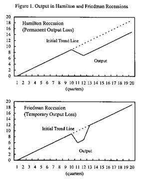
To recap, a Friedman recession is one which is associated with an increase in the output gap, which is the difference between potential output based on labour and capital capacity to produce. The Hamilton recession is where potential output itself is dropping, which signals a permanent loss in output.

The difference between the two can be illustrated by the following figure:

I thought at the time that this downturn would turn out to be of the Hamiltonian type, which requires an active fiscal policy response beyond automatic stabilizers, even if some of that effort leaks out through higher imports. A Friedman recession can usually be handled by judicious use of monetary policy alone.

Of course, it’s really hard to tell in the heat of the moment which particular situation you happen to be in, particularly with data lags of 2-3 months for some of the critical data. This is especially true since the defining variable – the output gap – is unobservable and has to be estimated.

Past experience and research output helps guide policy of course, so in the spirit of contributing to that, I’m going to take a rough and ready approach to answering this question. We’re still not quite out of the woods yet in terms of both global and Malaysian economic recovery, so this should be taken as just preliminary, not definitive.

In other words, it’s Friday evening, this is a purely academic exercise, and I’m amusing myself.

First, I’m going to take a purely stochastic (probability-based) non-model based approach i.e. I’m not even going to bother with estimating the output gap (that’s beyond my knowledge at the moment).

Many economic series typically display a consistent pattern – you can take advantage of this fact to model them stochastically by just following a mathematical rule (otherwise known as a “data-generation process” or d.g.p.) to define the shocks. Most follow a d.g.p. that approximates to a 1-lag auto-regressive pattern (denoted as AR(1)), which also implies what’s called trend-stationarity. In other words, if you take away the trend of an AR(1) time series, it will look like a random walk – the detrended time series is randomly distributed around a mean of zero.

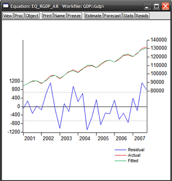
I’ve taken both nominal and real quarterly GDP for Malaysia for the sample period of 2001:1-2007:4 to illustrate what I mean. The regressions look like this:

rGDP = constant + @trend + d2 +d3 +d4 +AR(1)

nGDP = constant + @trend + d2 +d3 +d4 +AR(1)

…where @trend represents a linear time trend; d2, d3 and d4 are the seasonal dummies for 2Q, 3Q and 4Q of every year; and AR(1) is the autoregressive term.

Running the regressions yields:

All the explanatory variables are almost all statistically significant at the 95% level (Prob. values below 0.05), diagnostics all check out ok, and we have a very, very close representation of the actual time series (very high R2). It’s interesting to note that the error values (residuals) for the rGDP model are an order of magnitude smaller than that of the nGDP model.

Now that I have a baseline model(s), I can use historical values of GDP to forecast future values of GDP. This doesn’t turn out so well as a pure forecasting exercise because we had the commodity boom in 2008, and fell into recession in late-2008 to 2009 (out of sample forecast: 2008:1 to 2010:1):

Now you can partially see why so many forecasters and policymakers got caught out by this recession, and why so many risk models in the financial sector failed. The drop in output far exceeds the potential band of possible outcomes implied by historical data. That argues for a more structurally based approach to forecasting, though to be fair, that hasn’t fared much better in the present crisis.

But I digress. For today’s post, this failure serves my purpose pretty well – the forecasted level of GDP can be taken to represent potential output, and I now have a probability based measure of the output gap. I can’t obviously make a determination on whether there was a permanent drop in potential output, which defines a Hamilton recession, but what I can do with this is to ask (statistically speaking) whether there has been a change in the path of economic growth, which is almost (but not quite) the equivalent.

Specifically, assuming that productivity growth is about constant, then the trough of the recession represents a structural break and the economy would resume on its former trend from the new start point. Mathematically, I’m asking if there is a change in the intercept, while holding the slope of the regression more or less constant.

If the structural break as well as all the other variables are statistically significant, then I have proven my hypothesis that the Malaysian economy has moved to a permanently lower path of economic growth, and there has been a de facto loss in potential output. Bear in mind that we’re only looking at four quarters worth of data to work with i.e. from the point where the economy started growing again.

Defining d5 as the structural break variable, with values of 1 from 2001:1 to 2009:1, and zero thereafter, and rerunning the regressions with a larger sample range of 2001:1 to 2010:1, here are the results:

The results generated generally support my thesis – the economy has moved to a new path for economic growth, which in turn implies that there has indeed been a permanent loss in potential output.

Now for a more normative approach – it’s hard to reconcile my results with the fact that for Malaysia at least, the genesis for the recession was external. There was nothing fundamentally wrong with the economy pre-crisis, pace NEAC and the NEM. If demand was to fully recover, then we should expect to see a “V” shaped recovery back to trend (just back to the pre-crisis level of output is not sufficient). That hasn’t happened here, obviously.

In that light what I think we’re seeing is, potentially, a permanent loss in external demand and not a permanent loss in the potential output capacity of the economy. That in itself will eventually result in the same thing (unused capacity will be depreciate away), but there’s always hope for a stronger recovery though I’m having trouble right now seeing where that might come from.

So what could happen in time is more like a “U” shaped recovery back to trend – I’m crossing my fingers we don’t see a “W”. But in the context of what I’ve done here in this post, we’ll have to wait and see.

Technical Notes:

First graph and intellectual inspiration from:

Cerra, Valerie & Saxena, Sweta Chaman, "Did Output Recover from the Asian Crisis?", IMF Working Paper No. 03/48

Currencies: Tarred With The Same Brush

In Bloomberg today (excerpts):

Currency Controls Mount in Asia as Euro Hurts Exports

June 11 (Bloomberg) -- The world’s biggest expected swings in foreign-exchange markets and the euro’s record depreciation are prompting Asian exporters to seek currency controls.

TLtek Co., a South Korean exporter of auto-part making machines, called on policy makers to limit volatility caused by “gambling” on the won. Kuala Lumpur-based Sime Darby Bhd., the world’s biggest publicly traded palm-oil producer, needs to revise its business plan to account for the euro’s 19 percent drop against the ringgit. Taipei-based Maestro Innovations Corp., which makes infrared lamps for muscle pain, said curbs on the Taiwan dollar and China’s yuan would support orders.

Policy makers in South Korea, Taiwan and China are responding to Europe’s debt crisis by selling their own currencies, limiting investment inflows and delaying interest- rate increases. Goldman Sachs Group Inc. slashed its three-month Indian rupee forecast by 7 percent yesterday, Westpac Banking Corp. cut its year-end estimate for the won by 8 percent and ING Groep NV said the yuan won’t be revalued for a year.

“With the euro plunging, some central banks seem to be quite aggressive in stemming gains in their currencies,” said Kenichiro Ikezawa, who oversees about $3 billion as a fund manager at Daiwa SB Investments Ltd. in Tokyo and favors Brazilian and Australian debt over emerging-market Asian bonds. “China may delay revaluation and that, together with low yields in Asia, give little incentive to buy them.”

The South Korean won’s one-month implied volatility, a measure of exchange-rate swings used to price options, climbed 162 percent this quarter, the second-biggest jump among 47 currencies tracked by Bloomberg. Nine of the 10 biggest increases are in Asia. The won has the widest expected fluctuations at 24 percent, compared with 13 percent for the Indonesian rupiah and 12 percent for the Malaysian ringgit.

Exporters are seeking help from policy makers because the 10 most-active currencies in Asia outside Japan have strengthened an average of 19 percent against the euro this year. Shipments to the European Union fell in April from a month earlier, ranging from 5.6 percent for Malaysia to 19.5 percent for Thailand, according to government statistics. Europe took in 27 percent of India’s exports and 23 percent of China’s.

Sime Darby will have to revise its plans after the ringgit rose beyond 4 per euro for the first time since 2003, 13 percent stronger than its estimate, Chief Financial Officer Tong Poh Keow said in an interview on May 14 in Kuala Lumpur.

“We are doing our management plan and we will adjust based on our full-year expectations,” she said. “The decline in the euro will affect us.”…

…The Bank of Korea intervened at least twice in late May to stop the won gaining beyond 1,200 per dollar, a level 8 percent weaker than its 19-month high of 1,102 on April 26, according to traders who asked not to be identified as policy makers don’t discuss specifics of intervention. South Korea will introduce measures to reduce volatility in capital flows “soon,” Vice Finance Minister Yim Jong Yong said in a June 9 interview. The central bank will “act energetically” in the market to curb volatility, Governor Kim Choong Soo said today.

The Central Bank of the Republic of China (Taiwan) has stepped into the market to buy dollars almost every day in the past month, helping weaken the island’s currency by 1.6 percent to NT$32.35, said traders familiar with its operations, who also declined to be identified. In January, policy makers set a one- week deadline for money brought into the country to be invested or repatriated and in April ordered a review of loans to expose speculators. Governor Perng Fai-nan told reporters on June 4 the exchange rate will be “determined by market supply and demand.” …

…“Traders report Korea and Taiwan’s central banks have been in the market almost daily,” said Sean Callow, a strategist at Westpac in Sydney. “Ranges have been so wide over the past month and all the lines in the sand have been washed away.” …

…Bangkok-based Thai Union Frozen Pcl, the world’s second- largest tuna canner, wants the Bank of Thailand to restrain the baht to give it time to shift sales to “better markets,” President Thiraphong Chansiri said in a May 12 interview…

…Policy makers may seek to safeguard Asia’s growth potential by delaying rate increases, Tadashi Tsukaguchi, a fund manager in Tokyo at Sparx Group Co., the region’s biggest hedge fund with $7.3 billion in assets, said yesterday.

“A slowdown in Europe means countries like China, Korea and Southeast Asia have close to zero chance of raising rates,” said Tsukaguchi, who has taken short positions against some Asian currencies that profit from declines.

There’s no doubt that the fall in the Euro stemming from the zone’s ongoing fiscal problems will hurt local exporters. But the flip side to that is that a depreciation in the currency is one of the few mechanisms the Eurozone has to fend off complete economic collapse in the PIGS, which is in no one’s interest.

The action of China, Korea and Taiwan (there’s no mention of any of the other central banks among the countries affected) is tantamount to competitive devaluation, which really helps no one either.

Is BNM intervening in the market to depress the MYR? Not hardly – international reserves was virtually unchanged between April and May 2010, which means if there was intervention it was two-way. But current events do reinforce my belief that July’s Monetary Policy Meeting will see a pause in “normalisation” of the Official Policy Rate.

April 2010 Industrial Production

As April trade numbers have disappointed, so has industrial production (log annual and monthly changes; seasonally adjusted):

We’re going to see some revision in the consensus outlook for 2Q 2010 GDP growth based on these numbers, as its fairly clear that growth momentum is slowing. The Greek debt crisis in May will not help either, because part of the fallout has been a more rational valuation of commodities, fuel and non-fuel alike.

From examining the levels, it appears manufacturing is still in recovery mode, electricity generation is topping off (not a good sign for growth prospects), and mining is holding steady (2000=100; seasonally adjusted):

Most of the gains on the commodity-export front has been price-based, not volume-based, so the relative stagnation of mining output is not a worry.

On the other hand, it’s hard to tell where manufacturing is going because there is an overall surplus in capacity still (particularly in electronics), so external demand is the key factor here.

Electricity generation is partly consumer-based and partly industrial-based, so the slowdown here suggests the economic growth is also moderating, which was already evident in 1Q 2010. Much like in manufacturing, there’s a lot of surplus capacity in power generation (for the moment), so again this isn’t a supply constraint coming into play.

While I’d expect growth to pick up in May, I’m not holding my breath.

Quick Thoughts On The 10th Malaysia Plan

I haven’t read through the document yet, but I’ve got my hands on a nice summary (thanks, Abbas). Recall that the Malaysia plans outline (and only outline) the spending priorities of the government’s development budget over the next five year period (2011-2015). In addition to this, the 10MP also incorporates the implementation side of the New Economic Model, which has laid out some of the key strategies that are intended for the achievement of high income status by 2020.

I’ve made no secret that I don’t think high income status would be that hard to come by in the time frame allotted, nor that this status would be significant of itself. Under those circumstances, it’s more important to define the kind of economy and country we want to be, rather than the achievement of some nominal income figure that isn’t meaningful since it also requires the price level (and thus potential income inequality) to rise.

With that in mind, I’m framing my comments based on the key areas touched on:

1. Attracting Talent: It’s notable that many countries talk about halting their own “brain drain” and attracting “brain gain”, so we’re hardly alone in this area. There have been a lot of ideas and a lot of policies tried; but with very few exceptions, not much success. I really don’t see anything in the mooted policies and incentives here that will guarantee success – I think only a complete lowering of entry barriers and a really, really, really low level of income tax would be effective. On the other hand, success, as in a highly visible and concrete pace of economic growth and prospects, is its own virtue – if everything else works, so will this, but not before.
2. Enhancing Bumiputera economic participation: I was going to say that there’s not much change here, but looking at the figures, Bumi households aren’t that far off from the national median income (about 10% below). The key here is more on tackling income inequality. The 30% corporate equity figure is I think lip service to Perkasa and Bumi sensibilities, as I don’t think it’s really achievable in the foreseeable future. Ironically, the 10MP talks about emphasising institutional aggregation of investment funds via unit trust schemes, completely at odds with what Bursa Malaysia has been pursuing.
3. Raising Employment: 2.4% employment growth is lowballing the numbers required, which suggests that the unemployment target of 3.1% by 2015 is probably out of reach. The age cohorts entering the workforce over the next five years implies a required growth rate closer to 2.8%-3.0%. Did anyone actually model this, or were they working off of the crude birth rate?
4. Reforming the Labour Market: Lots to like here, and echoes the NEM. Easier hiring and firing might make the trade unions (and most workers) antsy, but reduces the cost of labour and increases efficiency. I love the pending change in employment regulation to regularise part-time employment, which would help both workers and employers (but implementation is always a bugbear). Increasing female labour force participation is something I’ve advocated for some time, although on deeper reflection, it’s something that will happen eventually due to the increased levels of participation for younger women. I think the allocation for the Relief Fund for Loss of Employment won’t be enough given the disruptions the change in development model will bring.
5. Infrastructure: My thoughts on broadband were posted this morning. Energy security by utilising coal and LNG isn’t terribly environmentally friendly.
6. Socio-economic development: Lots of targets, precious little in the way of effective policies, except the proposal for amalgamation of agricultural land which will unfortunately be conducted via RISDA and FELCRA. Where’s the profit motive? Let the private sector do this!
7. Social Safety Net/Special Target Groups: Not before time, this one. And it should make Sabahans and Sarawakians happier, or at least less upset.
8. Education System: Entry age for schooling lowered, and kids get even more pressured, but I think this is probably necessary for poorer households to catch up. Holding schools accountable is hypothetically great, but I’m wondering about implementation here. Has anybody tried this before, and what were the outcomes? Higher pay and better career paths for teachers is way overdue. Technical and vocational education in the mainstream? Yes!!
9. Vibrant Liveable Cities: I see potential for a lot of pork-barrel projects here.
10. Safety: Lots on enforcement, not so much on prevention except for improving rehab of drug addicts.
11. Valuing the Environment: This conflicts with the goals and policies planned for energy security.
12. The 12 NKEAs: I have little argument here, though I’m not too sanguine over the prospects in the broader agricultural sector, as long as there is a focus on smallholders. Cooperatives just won’t cut it.

Technical Notes

The 10th Malaysia Plan, Economic Planning Unit

Conflicts Of Interest: Bursa Malaysia Edition

No, this isn’t about BCorp and the do-they/don’t-they have a new sports betting license. I caught this on Bloomberg yesterday (excerpts, emphasis mine):

Malaysian Exchange Seeks to Lure Individual Investors

June 9 (Bloomberg) -- Malaysia’s bourse said it’s seeking to lure individual investors who have shunned the market a decade after the Asian financial crisis.

Bursa Malaysia Bhd. is working with brokerages and banks to “to reach out to retail investors in various towns and cities” to open up accounts and encourage online trading, Chief Executive Officer Yusli Mohamed Yusoff said in an interview in Kuala Lumpur.

Trading by individuals fell to as low as 20 percent of trading value from more than half before the start of the Asian financial crisis in 1997, when the benchmark index slumped by a record 52 percent.

“A lot of retailers lost a substantial amount,” Yusli said yesterday. The result is that the market is now “dominated by the local institutions,” he said.

Most individual savings started shifting to mutual funds and unit trusts since Malaysia’s economy went into a recession in 1998, Yusli said. They haven’t returned to stock trading even as the economy expanded at an annual average of 5 percent over the past decade and the benchmark index more than doubled...

...The exchange aims to boost the share of trading by individual investors “closer to a third,” tapping Southeast Asia’s second-highest savings rate, Yusli said, declining to give a target date. Malaysians saved 38 percent of gross national income in 2008, lagging behind only Singapore’s 47 percent, according to data compiled by the World Bank and Malaysia’s central bank.

The KLCI’s 45 percent gain last year lagged behind Southeast Asian neighbors even after the government announced stimulus plans totaling 67 billion ringgit ($20 billion) to help pull Southeast Asia’s third-largest economy out of a recession.

Trading slumped by half to an average $375 million a day over the six months ended May from the same period 13 years ago, right before the start of the regional financial crisis in July 1997, according to data compiled by Bloomberg. Neighboring Singapore’s figures have quadrupled to $1.1 billion over that time, data from the city-state’s exchange show...

...The slump in trading by individuals coincided with an exodus by foreigners from Southeast Asia’s second-biggest stock market, leaving Bursa more reliant on domestic institutional funds. Overseas investors have sold a net 1.36 billion ringgit of Malaysia’s equities this year, adding to 8.57 billion ringgit withdrawn in 2009 and 38.6 billion ringgit that flowed out in 2008, according to exchange data. In 2007, they bought a net 24.7 billion ringgit.

The exit left foreigners holding 20.6 percent of local stocks at the end of April, down from 27.5 percent in April 2007, according to stock exchange data. Overseas investors held 9.33 percent of Tenaga Nasional Bhd. at the end of April, compared with 27 percent in April 2007, according to data from Malaysia’s biggest power producer.

The state-controlled Employees Provident Fund accounts for 50 percent of daily trading volume in the equity and bond markets, Prime Minister Najib Razak said on March 30. More than half of the 417.1 billion ringgit of market value in the benchmark stock index is owned by government-linked funds, according to calculations by Bloomberg.

“We’d rather see a more balanced distribution, so that one particular sector doesn’t dominate the market so much,” Yusli said.

Retail investors’ share of trading is low by comparison with at least one neighbor, Thailand, where individuals accounted for 56 percent of turnover so far this year, according to data compiled by Bloomberg. Exchanges in neighboring Indonesia and Singapore don’t track the figures.

I can understand the argument regarding diversifying trading away from EPF. What I don’t get is why target individual investors, if trade diversification is really Bursa’s goal.

Theory suggests that the costs of diversifying portfolio risk is lower when individuals invest via unit trusts, and information costs for individuals are then relegated to just monitoring the fund manager(s) and the overall market, rather than a personal stock portfolio. Menu costs are lower as well, in terms of adjusting the portfolio mix based on market conditions. In addition, institutional funds are (supposedly) better able to handle market volatility and have a better chance to monitor and evaluate individual stocks (with some reservations).

The problem Bursa is facing is that while Malaysia does indeed have a nominally high savings rate, these savings are by private enterprises and not by households. That’s means that Bursa’s effort is probably doomed to fail, and thankfully so – given the reasons I outlined above, there’s not much benefit in aggregate for individual investors to put funds directly into the market. And I’d not be very happy if Bursa started targeting corporate savings either – investing in the stock market should not be part of corporate business activity.

Why I’m calling this a conflict of interest on Bursa’s part is because of their corporatised structure, and because of the benefits that individual investors can bring to market activity. That line about the fall in daily trading volume is key to understanding this – who benefits most from higher trade volume? Stock brokers and by extension, Bursa itself; certainly not individual investors, who tend to be market followers rather than market leaders. The fact that Bursa Malaysia is a publicly listed company and answerable to shareholders means that their incentives are highly skewed toward increasing revenue and profits, rather than safeguarding individual investor interests.

As I say, they aren’t likely to succeed, but the very fact they’re pursuing this course is disturbing.

We Are Not Alone: Developing World Fuel Subsidies

The OECD released this press release yesterday (excerpts, emphasis added):

Global warming: ending fuel subsidies could cut greenhouse gas emissions 10%, says OECD

09/06/2010 - Careful phasing-out of fossil fuel subsidies can be a low-cost way to meet part of the targets announced following the U.N. climate conference in Copenhagen. According to new OECD analysis based on data from the International Energy Agency (IEA), ending fossil fuel subsidies could cut global greenhouse gas emissions by 10% from the levels they would otherwise reach in 2050 under “business as usual.

This would make economic sense as governments strive to cut budget deficits in the wake of the financial and economic crisis. That is why G20 leaders agreed when they met in Pittsburgh in September 2009 to “rationalize and phase out over the medium term inefficient fossil fuel subsidies that encourage wasteful consumption” and requested the OECD, along with the IEA, OPEC, and the World Bank, to prepare a joint report for the G20 Summit later this month in Toronto.

“Many governments are giving subsidies to fossil fuel production and consumption that encourage greenhouse gas emissions, at the same time as they are spending on projects to promote clean energy,” said Angel Gurría, OECD Secretary-General. “This is a wasteful use of scarce budget resources.”

The IEA has estimated that subsidies to fossil fuel consumption in emerging and developing countries amounted to USD 557 billion in 2008. Some estimates suggest that fossil-fuel producer subsidies could amount to as much as USD 100 billion per year. However, estimates in developed countries are harder to obtain because they are often transferred in indirect ways, which makes them no less important. The OECD is working to fill these data gaps, and also to develop an accounting framework and agreed methods for estimating different support elements...

...Tax exemptions for diesel fuel use in mining, agriculture and fisheries are common in many countries. In OECD countries alone the value of these tax preferences amount to approximately USD 8 billion each year for farmers and a further USD 1.1 billion each year for the fishing industry (see examples of selected tax expenditures of fossil fuel production or use in OECD Countries).

Many subsidies to fossil fuels are also inefficient in achieving their intended objectives of supporting the poor in countries without adequate social security systems. They typically benefit richer rather than poorer households, as poor people, for example, often cannot afford cars. Better targeting these subsidies to those who most need them can improve welfare of the poor and benefit the environment at a lower budgetary cost...

...Key elements in successful reform include: announcing subsidy phase-out plans early; phasing them in gradually; ensuring transparency and raised awareness by publicly circulating information on who pays and who benefits from reform; and accompanying reforms with measures to limit negative impacts on poorer households.

Everything PEMANDU said last month and more.

Appealing For Research-Based Policy Design

In my email inbox today (abstract, emphasis mine):

Home Computer Use and the Development of Human Capital

This paper uses a regression discontinuity design to estimate the effect of home computers on child and adolescent outcomes. We collected survey data from households who participated in a unique government program in Romania which allocated vouchers for the purchase of a home computer to low-income children based on a simple ranking of family income. We show that children in households who received a voucher were substantially more likely to own and use a computer than their counterparts who did not receive a voucher. Our main results indicate that that home computer use has both positive and negative effects on the development of human capital. Children who won a voucher had significantly lower school grades in Math, English and Romanian but significantly higher scores in a test of computer skills and in self-reported measures of computer fluency. There is also evidence that winning a voucher increased cognitive ability, as measured by Raven's Progressive Matrices. We do not find much evidence for an effect on non-cognitive outcomes. Finally, the presence of parental rules regarding computer use and homework appear to mitigate the effects of computer ownership, suggesting that parental monitoring and supervision may be important mediating factors.

What this means is that just giving computers to kids at home is not a sure-fire way of improving educational outcomes – parental guidance is a necessary adjunct. This goes against the conventional wisdom that just having a computer in the home make kids smarter, by allowing them to be more computer literate. This paper affirms that computer literacy rises, but at the potential cost of reducing the impact of education in other fields of study.

The reason why I’m bringing this up together with policy design, is this report a couple of weeks back (extract):

One million free laptops for poor students

RAUB: One million laptop computers will be given out free to poor students of secondary schools throughout the country to increase broadband penetration in the country.

Malaysian Communications and Multimedia Commission (MCMC) chairman Tan Sri Khalid Ramli said the Government was targetting a penetration level of 50% by the end of the year.

“At the moment, the country has achieved 36% broadband penetration,” he said after attending the World Telecommunication and Information Society Day celebration in the Tersang 3 Felda scheme near here yesterday.

The reason for pushing for broadband penetration is because research indicates that higher broadband penetration can improve economic growth. But the degree of causality and the transmission mechanisms between higher broadband penetration and economic growth really needs to be looked at, before a policy is set to shoot for targets.

It’s no use just giving out free laptops and broadband access to poor kids, if the actual mechanism by which higher broadband penetration improves the economy is through reducing communication costs and lowering barriers between businesses, or between businesses and consumers. And its an even worse policy if it backfires and reduces educational outcomes for the young.

Going for increased broadband penetration (and hence, a hoped for increase in national output) by just giving away laptops, is a triumph of form over substance – unless there are backup mechanisms to ensure that the policy goals are actually met. I don’t see that here.

Technical Updates

Ofer Malamud, Cristian Pop-Eleches, “Home Computer Use and the Development of Human Capital”, NBER Working Paper No. 15814, March 2010

Debt and Subsidies Clarified

What with the brouhaha over the actual amount of subsidies being paid, and the actual amount and definition of “national debt” as reported yesterday, PEMANDU felt it had to step in with clarification (in full from The Star):

Subsidy figures are correct, says Pemandu

PUTRAJAYA: Both sets of subsidy figures released by the Treasury and the Performance and Delivery Unit (Pemandu) are correct, the unit said in a statement.

It said the Treasury had only focused on direct subsidies because it took a public finance management approach in defining subsidy while the Pemandu lab had taken a macro-economic approach.

“The approach includes both direct and indirect subsidies as a necessary measure to increase competitiveness and remove market distortions,” it said here yesterday.

The Treasury had on Tuesday in a briefing to backbenchers announced total subsidies at RM18.6bil last year while Pemandu’s lab findings put the figure at RM74bil.

The unit said the definition of subsidy by Pemandu’s lab was based on that provided by the Organisation of Economic Co-operation and Development (OECD) in 1996.

“Some of these subsidies include contract obligations, financial support and rebates, assistance to Ministry of Finance Incorporated companies, and cost-based financial assistance which includes emolument for education and health.

“The substantial items under indirect subsidies which are not covered by the Treasury include cost-based financial assistance, assistance to MoF Incorporated companies and gas subsidy. “The subsidies defined by the Treasury are those which affect the Federal Government balance sheet directly,” it said.

The unit reiterated that as a gross domestic product (GDP) percentage, Malaysia continued to be one of the highest subsidised countries in the world, even higher than Indonesia and the Philippines.

“On average, the OECD subsidy level is 1.5% of the country’s GDP. Both the Treasury and Pemandu agree that Malaysia should increase its revenue or GDP and at the same time, reduce government expenditure in the next 10 years in order to stay competitive,” it said.

The unit said the Government would also continue to fight corruption, reduce wastages and leakages based on the Auditor-General’s report to reduce overall expenditure besides removing subsidies.

It said it also wished to clarify that the country’s national debt stood at RM234bil, which is defined as external debt and inclusive of both public and private debt.

“Our government debt stands at RM362bil, comprising domestic debt (96%) and foreign debt (4%).”

A Matter of Definition

When this report first came out yesterday afternoon, I thought it was a typo. But it turned up on the front page of the NST today in big bold letters, so someone has a very different idea of what “national debt” means than I do (excerpt, emphasis added):

Debt under control

KUALA LUMPUR: Malaysia’s debt is under control and steps are being taken to reduce it to prevent the country from suffering the same fate as Greece and Iceland.

Prime Minister Datuk Seri Najib Razak said last year, the country’s debt fell almost one per cent to RM233.92 billion from RM236.18 billion in 2008. This is because of the repayment of some loans and the stronger ringgit against the US dollar.

The budget deficit is also expected to drop and is under control in the medium and long term.

“These measures will ensure that the federal government’s deficit does not rise to the extent that we will be unable to settle our debt,” he told the Dewan Rakyat yesterday.

The government will reduce its external debt by tapping domestic loans because local investors are flush with money and the cost of borrowing is also cheaper. Malaysia also has a comprehensive system that detects financial risks and weaknesses early.

Here’s the coverage from The Star, in case NST changes the link.

I’ve always taken “national debt” to mean the total outstanding borrowing of the national government, which are the collective liability of all the country’s citizens. It appears in Malaysia’s case, “national debt” is something completely different – it’s the aggregate external debt of the country, comprising government, semi-government and private sector (source: 4Q 2009 Treasury quarterly economic report, pg 14-16).

The trouble is partly the way the news was reported (it appears to conflate “national debt” with government debt), and partly from the PM’s further comments on the subject – if you check the actual breakdown, direct external government debt is just RM13.8b, or 5.9% of the total. The bulk of this “national debt” comprises RM71.6b from Non-Financial Public Enterprises (NFPEs), RM70.0b from the private sector, and RM69.0b from the banking system. Of these amounts, only the NFPEs (e.g Petronas) could be said to fall under direct government influence. So talking about consolidating the federal government deficit is more than a little disingenuous, because it has almost no bearing over reducing the “national debt” as it is curiously defined here.

Mankiw On Pigovian Taxes

I believe, given the costs to Malaysian society that come from excess consumption of sugar, that not only should subsidies and price controls on it be dropped but that it should also be taxed as well. The argument goes double for petrol, as the impact on society and the environment are that much greater.

N Gregory Mankiw provides both sides of the debate in this NYT article (excerpts):

Can a Soda Tax Save Us From Ourselves?

AS governments large and small face sizable budget shortfalls, policy makers are looking for ways to raise tax revenue that will do the least harm and, perhaps, even a bit of good. One idea keeps popping up: a tax on soda and other sugary drinks…

…Economists have often advocated taxing consumption rather than income, on the grounds that consumption taxes do less to discourage saving, investment and economic growth. Hence the case for broad-based consumption taxes, like a value-added tax. The main issue for the soda tax, however, is whether certain forms of consumption should be singled out for particularly high levels of taxation.

One argument for specific taxes is that consuming certain products has an adverse impact on bystanders. Economists call these effects negative externalities.

Taxes on gasoline can be justified along these lines. Whenever you go out for a drive, you are to some degree committing an antisocial act. You make the roads more congested, increasing the commuting time of your neighbors. You increase the likelihood that other drivers will end up in accidents. And the gasoline you burn adds to pollution, including the greenhouse gases thought to cause global climate change.

Many economists advocate gasoline taxes so that drivers will internalize these negative externalities. That is, by raising the price of gasoline, a tax would induce consumers to take into account the harm they cause after making their purchases. One prominent study added up all the externalities associated with driving and concluded that the optimal gasoline tax is over $2 a gallon, about five times the current level (combining the federal and a typical state’s levies) and about the tax rate in many European countries.

Applying that logic to other consumer goods, however, is not as straightforward. Consider cigarettes. They are among the economy’s most heavily taxed products, as governments try to discourage people from smoking. Yet the case for such a policy cannot rely on a conventional externality argument.

When a person sits at home and smokes two packs a day, the main adverse impact is on his or her own health. And even if second-hand smoke is a concern, that problem is most naturally addressed within the household, not at the state or federal level.

Sometimes, advocates of “sin” taxes contend that consumers of certain products impose adverse budgetary externalities on the rest of us — that if the consumption induces, say, smoking- or obesity-related illness, it raises health care costs, which we all pay for through higher taxes or insurance premiums.

Yet this argument has a flip side: If consumers of these products die earlier, they will also collect less in pension payments, including Social Security. Economists have run the numbers for smoking and often find that these savings may more than offset the budgetary costs. In other words, smokers have little net financial impact on the rest of us…

…There is, however, an altogether different argument for these taxes: that when someone consumes such goods, he does impose a negative externality — on the future version of himself. In other words, the person today enjoys the consumption, but the person tomorrow and every day after pays the price of increased risk of illness.

This raises an intriguing question: To what extent should we view the future versions of ourselves as different people from ourselves today?

…But people do not suddenly mature at the age of 18, when society deems us “adults.” There is always an adolescent lurking inside us, feeling the pull of instant gratification and too easily ignoring the long-run effects of our decisions. Taxes on items with short-run benefits and long-run costs tell our current selves to take into account the welfare of our future selves.

IF this is indeed the best argument for “sin” taxes, as I believe it is, we are led to vexing questions of political philosophy: To what extent should we use the power of the state to protect us from ourselves? If we go down that route, where do we stop?

Taxing soda may encourage better nutrition and benefit our future selves. But so could taxing candy, ice cream and fried foods. Subsidizing broccoli, gym memberships and dental floss comes next. Taxing mindless television shows and subsidizing serious literature cannot be far behind.

Even as adults, we sometimes wish for parents to be looking over our shoulders and guiding us to the right decisions. The question is, do you trust the government enough to appoint it your guardian?

N. Gregory Mankiw is a professor of economics at Harvard.

I think from my point of view, that the answer to that philosophical question is this: you apply taxation or subsidies when the public costs or benefits are large and obvious. That’s one basic argument for the provision of public goods like healthcare and defence, and for monopolies like rail and electricity generation. Taxing sugary foods and drinks might not meet that criteria, but taxing sugar itself does.